Agent-Based Swarm Model

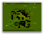
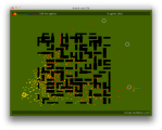
Swarming agents that seek a target, navigate through terrain (with fairly primitive means), avoid potential predators, starve, die, eat prey and carcasses. Misc emergent behaviour ensues. With a maze generator to produce a wide range of terrain structures.

Agents are coloured by generation (i.e., according to the time they were spawned), but lose saturation after some time as they start to starve. They will aim for one of three target points which is selected at spawn time. They can survive (and grow) by eating smaller agents, or taking a bite off a carcass.

Agents will avoid larger live agents, and carcasses when they’re not hungry
(the repelling force is a power law distribution relative to agent sizes),
but they won’t notice walls until they hit them, and then bounce off or get
stuck.

There is a limit to the total number of live (and dead) agents on screen.
Once the limit has been reached, new agents can only be spawned when any
agent reaches their target and is removed. (For this reason targets can
also be considered “breeding grounds”.)

Press the “f” key to toggle “flypaper mode“, which makes agents stick to
walls and die instantly. In this mode complex terrains are much harder to
navigate. Since agents will avoid larger carcasses these now act as “beacons”
for nearby walls, and allow new agents to travel farther.

A few histograms show live/dead/arrived agent counts per generation. This
allows to observe how quickly agents manage to find their target, a function
of the terrain. The target histograms are especially interesting in flypaper
mode, where it may take a few generations of dead “beacon” agents to mark a
path along walls until new agents can pass.

Terrain Models and Navigation

Press the space bar to start again with a new terrain. The basis of these
generated terrain models is a graph-based depth-first maze generator that involves a few additional steps to modulate terrain structures (e.g. wall strengths.) A post-processing step may remove random
walls between cells of the maze. A number of terrain types exist, and each new terrain will be a variant of one of these preconfigured types.

Agents navigate through the combination of a few primitive behaviours. They will aim towards their target, avoid colliding with other agents, escape the proximity of potential predators (larger agents), and avoid carcasses unless they are hungry. These agent interactions rely on distance computations and power-law, which allows for a certain degree of prediction. Wall interactions lack any predictive quality; agents cannot perceive walls until they reach them, and then bounce off in random directions or (in flypaper mode) get stuck. A fair amount of time was spent fine-tuning the intensity and interaction of these behaviours in various terrains.

A big limitation of this is the absence of any “line of sight” logic, and of stronger predictive and planning behaviours. As a result agents will e.g. head in the direction of their target even with walls between them, and they will get stuck in corners without the ability to find reasonable alternative routes.

Examples of Emergent Behaviour

With more complex terrains it is worth letting the model run for a few minutes to observe emerging zones. Let’s look at an example of how the system evolves in flypaper mode, broken down into stages.

The start of a new terrain. Agents get stuck on walls and die, start covering larger and larger areas of it; since live agents will avoid dead ones (unless they are hungry) these carcasses now act as wall beacons.

On the left of the terrain agents started assembling in a bay. To the right of the bay the terrain blocks direct access to their targets, and a wall at the top of the bay prevents them from escaping. Any agent that arrives here by itself would be trapped. However agents will avoid colliding with other agents, and will attempt to avoid the close proximity of predators (larger agents), and in combination this results in complex flows and eddies. Once enough agents are part of this flow some agents may get pushed over the edge of the bay, to then slowly build a longer path for later generations, step by step.

Over a period of a few minutes, as agent carcasses begin to cover most of the wall space between the origin and the three target points, live agent numbers steadily decrease. All three target points can now be reached, which allows a process of renewal to take place: every agent that reaches their target allows a new agent to be spawned.

If agents are “bullied” into a detour towards their target they may still encounter open wall space in less-covered areas once they can escape. E.g. a forced clockwise tour around the terrain towards the bottom-right target will lead to some open wall patches in the top right corner of the terrain.

A few minutes later (not shown here) all live agents are of a recent generation, which implies all new agents either reach their target, get eaten, or get stuck and die; all of which allows new agents to be spawned. Agents that are temporarily stuck in bays will not stay there for long, and their presence allows others to pass. The population count has decreased again, but not by much; we may be heading towards a stable state.

About half an hour after starting the simulation the population count appears to remain in the 30-40 range. A delicate equilibrium.

The broad range of agent interactions and emergent behaviour that can be observed, including the examples mentioned above:

• The distribution of colour across the terrain indicates zones of faster or slower propagation.
• Groups of agents may push other (smaller) agents in wrong directions away from their target until they get a chance to escape. These “bullied” agents will wiggle their beak as they continuously attempt to change direction.
• Dense clusters between walls result in complex flows, and agents may start panicking as there is no space to evade nearby predators.
• Dead ends may result in starvation deaths, which provides food to grow. This allows a few agents to escape once they have become large enough to move in larger steps.
• Also note the interaction between walls and carcass prey in flypaper mode: an agent may be tempted to eat a wall beacon carcass to survive, but this brings it in closer proximity with the wall, and makes it possible that it will itself get stuck and die. This could be regarded as a form of “weary desperation”.
• The system may reach an equilibrium where many agents are stuck or dead, but targets are still accessible enough so that there is a steady trickle of renewal. Such equilibria may have any number of live agents.

The Processing source is on GitHub.

CA with Periodic Reorganisation

Multiple cellular automata interleaved with periodic processes of reorganisation:

• Randomly move some tiles.
• Fill all tiles with their dominant colour.
• Rearrange all tiles in circular order.
• Sort all rows by colour.

The Processing source is on GitHub.

Visualisation of London Cycle Hire Flows

The London Cycle Hire scheme has docking stations across the inner city where bicycles can be picked up and returned. Their system records the time of checkout and return, along with a docking station identifier.

The video below visualises these flows. The focus is on the local density of cycling activity, and on docking station activity (checkouts and returns) over time. It e.g. shows clearly that activity in the morning hours is predominantly constituted of cycle trips from outer city areas to the centre.

• Bike stand size: estimated inventory; or rather, cumulative growth since start of day: all incoming minus all outgoing bikes.
• Bike stand hue: gain/loss of bicycles within the last ~2h (green: gain, red: loss, yellow: no change.)

The Processing source is on GitHub.

Eye Candy: Cellular Automaton

A simple 1D CA. Starts with a random seed, then continues to produce new generations until encountering a repetition of an old state. Rinse, repeat. Sadly no indication that it may exhibit “Rule 110“-style behaviour.

The Processing source, as usual, is on GitHub.

Visualisation of Geo-Coded Event Stream Data

A visualisation of an event stream of geo-coded tweets. This application aggregates geographic points in a grid, and produces a 3D bar chart of intensity levels. Use the mouse to rotate the scene, and to select events on a timeline histogram. Optionally make use of filters to only display subsets of the data (retweets, tweets from specific Twitter clients, tweets in specific languages.)

The Processing source comes with a sample data set.

Visualising Structured Data on Geographic Maps: Evaluating a Hexagonal Map Visualisation

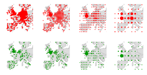
An important aspect of spatial analysis is the choice of appropriate forms of representation. Choropleth maps are an appropriate, widely-used representation for univariate spatial data sets; but how can data distributions be visualised on geographic maps? I.e., how can one visualise data that has spatial, categorical, and quantitative aspects?

We developed a map-based histogram based on a hexagonal tessellation scheme and will evaluate it with geometric and spatial analysis techniques. Such visualisations can be used to illustrate e.g. cultural differences, as demonstrated here with a data set on language-specific colour naming preferences. Exemplary questions of this data may be: what are the most popular colour categories within a country? How fine or broad are the colour categories for particular hues? Do Spanish-speaking respondents have more fine-grained colour name categories for orange tones than English-speaking ones?

In developing such a visualisation there are a number of challenges to overcome which we will outline below. A fundamental question is whether we can illustrate spatial, categorical, and quantitative aspects (country association, colour names, and colour frequencies) without introducing needless visual clutter. In Edward Tufte’s terms: we will strive for a high data-ink ratio.

Get the report: Hexagonal Maps 2011-12-16

Eye Candy: Sprite Oscillation

A simple sprite oscillation system involving rhythms of small primes, and rendering feedback loops. Coefficients (36, 35, 32, 24) taken from La Monte Young‘s “The Second Dream of the High-Tension Line Stepdown Transformer”. Very addictive. The Processing source requires the GLGraphics library.

Eye Candy: Particle System

A simple particle system involving rhythms of small primes, and rendering feedback loops. The Processing source requires the GLGraphics library.

This Space Intentionally Left Blank

Bear with us as we get started.